6 Introduction to the GDAL library

GDAL (Geospatial Data Abstraction Library) is an open source, MIT-licensed library which is a collection of functions used to convert between different vector and raster GIS formats, data types, and coordinate reference systems (the PROJ.4 library is integrated into the GDAL library). Besides this, GDAL contains other functions for manipulating raster data. In the following, its functionality will be illustrated through several examples.

Hence, using the GDAL library, vector data can be converted from one coordinate system to another and from one format to another. Using cartographic projections with vector data is simple, the conversion is carried out point by point, and examples for points are given in the decription of the PROJ.4 library.

Using the ogrinfo function, basic information on the vector file can be obtained.

ogrinfo -so test.kml test
INFO: Open of `test.kml'
      using driver `LIBKML' successful.

Layer name: test
Geometry: Unknown (any)
Feature Count: 1
Extent: (20.476164, 44.805681) - (20.476164, 44.805681)
Layer SRS WKT:
GEOGCS["WGS 84",
    DATUM["WGS_1984",
        SPHEROID["WGS 84",6378137,298.257223563,
            AUTHORITY["EPSG","7030"]],
        AUTHORITY["EPSG","6326"]],
    PRIMEM["Greenwich",0,
        AUTHORITY["EPSG","8901"]],
    UNIT["degree",0.0174532925199433,
        AUTHORITY["EPSG","9122"]],
    AUTHORITY["EPSG","4326"]]
Name: String (0.0)
description: String (0.0)
timestamp: DateTime (0.0)
begin: DateTime (0.0)
end: DateTime (0.0)
altitudeMode: String (0.0)
tessellate: Integer (0.0)
extrude: Integer (0.0)
visibility: Integer (0.0)
drawOrder: Integer (0.0)
icon: String (0.0)

The -so parameter is given to show only the summary data about the file, without listing all entities; this is followed by the file and layer names, usually identical to the file name without the extension. If the -so command is given without parameters, then the section relating to the vector entities’ geometry would added to the previous output:

OGRFeature(test):1
  tessellate (Integer) = -1
  extrude (Integer) = 0
  visibility (Integer) = -1
  POINT (20.4761644699725 44.8056810018923)

If we want to transform this file into ESRI Shapefile format or the Gauss-Krüger projection for Serbia with the Hernannskogel datum, the ogr2ogr command would be used with the following parameters:

ogr2ogr -f "ESRI Shapefile" testGK.shp -t_srs "+proj=tmerc +lat_0=0 +lon_0=21 +k=0.9999 +x_0=7500000 +y_0=0 +ellps=bessel +towgs84=574.027,170.175,401.545,4.88786,-0.66524,-13.24673,6.89 +units=m" -s_srs "EPSG:4326" test.kml

The parameter -f defines the output format, and the list of all formats can be obtained using the ogr2ogr –formats command. This is followed by the resulting file’s name; -t_srs is the argument used for defining the target coordinate system using the PROJ.4 notation or EPSG code; -s_srs is the definition of the input file’s coordinate system, which can be omitted if it is contained in the file itself. It should be noted that when the ESRI Shapefile is used and accompanied by a .prj file, then, the datum parameters are not written in the description and need to be defined again. This is often the case for other datum-related formats not defined by the EPSG code. After the command comes the input file’s name. A summary description of the new file is given as follows:

ogrinfo  testGK.shp testGK
INFO: Open of `testGK.shp'
      using driver `ESRI Shapefile' successful.

Layer name: testGK
Metadata:
  DBF_DATE_LAST_UPDATE=2018-02-09
Geometry: Point
Feature Count: 1
Extent: (7458993.628067, 4962479.113279) - (7458993.628067, 4962479.113279)
Layer SRS WKT:
PROJCS["Transverse_Mercator",
    GEOGCS["GCS_Bessel 1841",
        DATUM["unknown",
            SPHEROID["bessel",6377397.155,299.1528128]],
        PRIMEM["Greenwich",0],
        UNIT["Degree",0.017453292519943295]],
    PROJECTION["Transverse_Mercator"],
    PARAMETER["latitude_of_origin",0],
    PARAMETER["central_meridian",21],
    PARAMETER["scale_factor",0.9999],
    PARAMETER["false_easting",7500000],
    PARAMETER["false_northing",0],
    UNIT["Meter",1]]
...

However, the same logic cannot be applied to raster data as will be illustrated in the following example. Suppose we are converting raster data given in geographic coordinates into an equivalent Sinosoidal projection, using the method of first converting each pixel into a polygon and then carrying out a vector transformation, Figure 6.1.

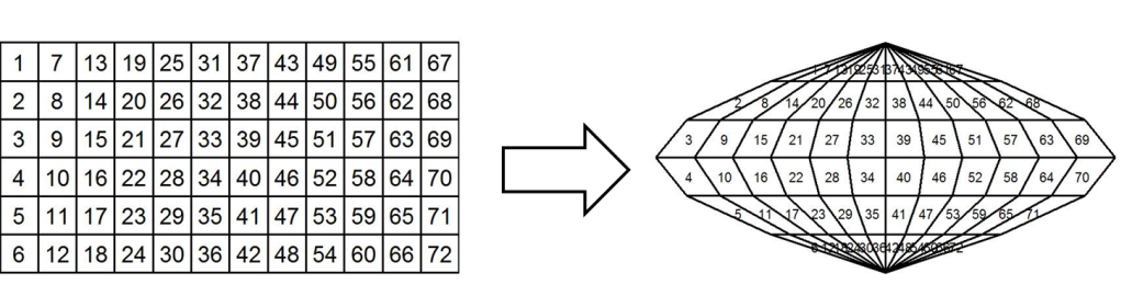
Figure 6.1: Simulation of a vector approach to raster coordinate transformation.

Pixels are arranged as rectangular elements, with all pixels having the same geometry. It is necessary for the transformed raster to have a pixelated structure in which all pixels have the same geometry as well. From the previous example it is clear that this cannot be achieved since pixels are deformed because of the characteristics of the projection; hence, they do not represent rectangular elements.

In raster transformations, it is necessary to again achieve a raster structure; however, in doing this, another problem can arise. Namely, pixels can be mapped outside of the area encompassing the Earth’s surface (a Wraparound Problem), Figure 6.2.

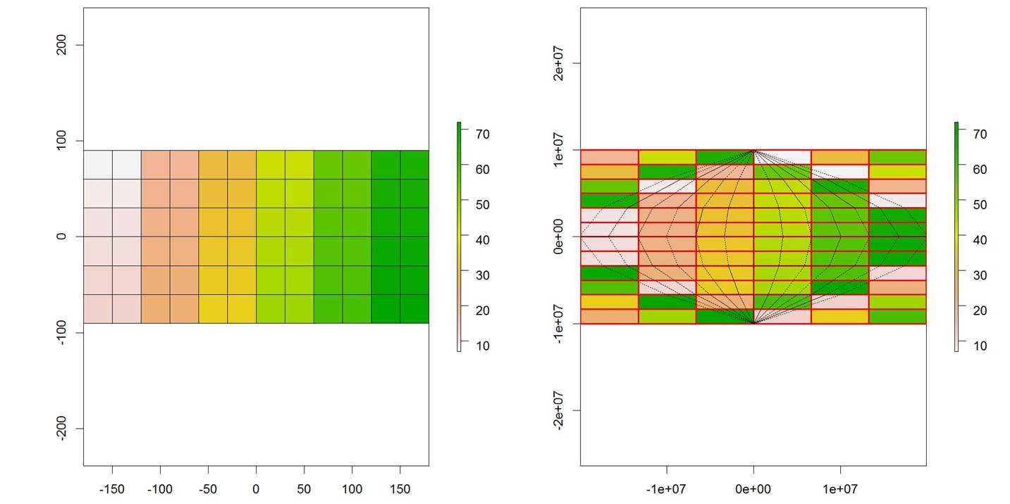
Figure 6.2: Raster transformation and example of a Wraparoung problem.

Finally, the transformation for the previous example is shown in Figure 6.3.

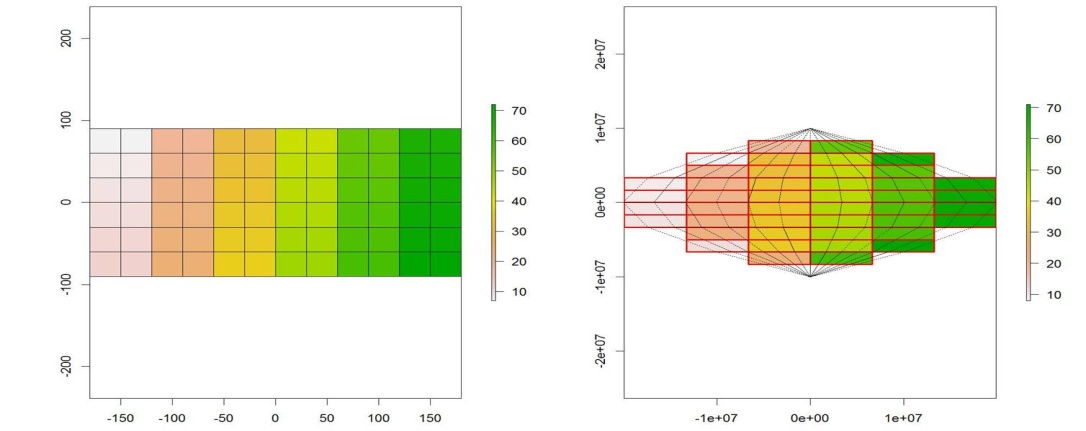
Figure 6.3: Raster transformation with a solution to the Wraparound problem.

From previous figures, it can clearly be seen that the position and number of pixels are not the same in both projections, and that the pixel values are rearranged so as to represent the positions and values of input pixels as closely as possible. Methods that secure the rearrangement of pixel values from the input raster to the output raster are called resampling methods. Here, some of the resampling methods will be briefly mentioned.

The Nearest Neighbor resampling method is a simple resampling method. It takes into account the nearest pixel center from the input raster in relation to the output raster pixel centers, so that it finds the nearest neighbor and assigns it the original input pixel’s value. The method is used when it is necessary to perform a quick resampling, as well as with categorical or normalized data.

Bilinear interpolation takes into account the four nearest cells in the direction of the raster’s main axes, and calculates the values of the output raster as the average value of the nearest cells.

Cubic convolution is similar to the bilinear method but the averaging is performed on 16 adjacent cells.

An example of using the gdalwarp function is illustrated on Natural Earth data which represent continents and bodies of water, with stilyzation integrated into a TIFF file.

gdalwarp -t_srs '+proj=sinu +lon_0=0 +x_0=0 +y_0=0 +datum=WGS84 +units=m +no_defs' -r cubic -co COMPRESS=LZW -dstalpha NE1_50M_SR_W.tif NE1_50M_SR_W_sin.tif

The -t_srs parameter is used to define the output file’s coordinate system, -r is used to define the resampling method (here, cubic convolution is chosen), -co is a parameter defining the compression method, and -dstalpha makes the pixels without an assigned value be displayed as transparent. The input file, NE1_50M_SR_W.tif, is shown in Figure 6.4. Unlike vector functions, for raster functions, the output file is always the last parameter in the function, NE1_50M_SR_W_sin.tif, Figure 6.5.

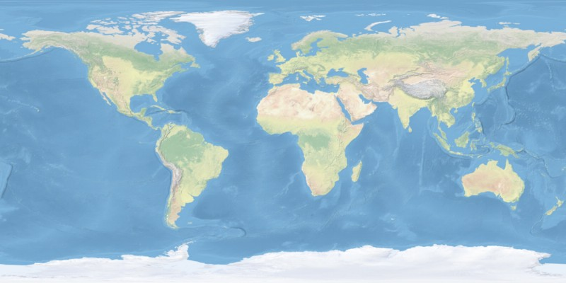
Figure 6.4: Display of continents in the WGS84 coordinate system, NE150MSRW.tif.

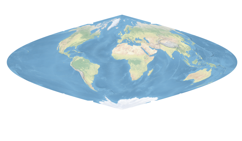
Figure 6.5: Display of continents in a Sinusoidal projection, NE150MSRWsin.tif.