7 Databases of spatial data

A database is a collection of structured data. The DataBase Management System (DBMS) is a software package which enables users to use, maintain, and manage databases. Databases are usually larges sets of data organized into tables. DBMS supports queries defined by declarative programming, such as SQL (Structured Query Language).

A relational data model is a data structure with defined attributes, series of attributes representing rows (tuples), and relations between attributes. When referring to extracting data from the databases, the term query is used, and when queries are used to change the database content, then the term transaction is used.

Databases of spatial data are databases that support a special type of data within tables (attributes, column defining geometry). Hence, with these databases, columns can be designated to represent spatial data. Besides, these databases also enable spatial queries, as well as spatial indexing of data using declarative programming, such as SQL. Databases of spatial data are not only systems for storing spatial data, but much more, as they are usually relational databases.

A simple example of a relational database is illustrated with three interconnected tables regarding plot ownership and owner information.

Personal_data

Personal_ID	Last_Name	First_Name	Date_of_birth
1234	Marković	Marko	01/01/1983
5678	Laban	Luka	02/05/1963
4321	Petrović	Petar	08/05/1973

Plot_information

PlotNumber	Geometry	Area
55	POLYGON(751….)	77
57	POLYGON(752….)	5
88	POLYGON(749….)	8

Owner_information

Plot	Owner	DateOfOwnership
57	5678	10/10/2015
88	4321	11/11/2016
55	1234	05/08/2013

This database consists of three tables. The first table has four attributes, and the other two have three. The attributes are organized in columns and rows represent strings of attributes (tuples). In each table, the attribute representing the key is given in boldface. The key is used to define the relations between tables, based on the common attribute. With common attributes it is easy to link two or more tables.

Databases have a defined scheme which defines attributes and data types reserved for storing attribute values. A maximum attribute length is usually also defined, e.g., by reserving a type for storing characters (strings) for the Last Name attribute with a maximum length of 20 characters. The scheme is illustrated below:

Personal_data (Personal_ID: [number,10], Last_Name: [string,20], First_Name: [string,20],  Date_of_birth: date)
Plot_information (PlotNumber: [number,8], Geometry: polygon, Area: [number,150])
Owner_information (Plot: [number,8], Owner: [number,10], DateOfOwnership: date)

Basic SQL commands are given without detailed explanations:

CREATE TABLE – creating a table in the database,
DROP TABLE – deleting a table from the database,
ALTER TABLE – changing the definition of a table,
CREATE INDEX – creating an index,
DROP INDEX – deleting an index,
CREATE VIEW – creating a view,
DROP VIEW – deleting a view,
SELECT – displaying the desired content from one or more tables,
UPDATE – changing table column values,
DELETE – deleting rows in a table,
INSERT – adding rows in a table,
GRANT – adding authorization on database objects to other users by the owner,
REVOKE – revoking authorizations given using the GRANT command.

If we want to show all plots with areas larger than 5 acres using SQL, the query should look like the following:

SELECT * FROM Plot_information WHERE Area > 5

The * character is used when the query relates to every row in the table. Similarly, a query can be defined to display plot and owner information together.

SELECT * FROM Plot_information, Owner_information WHERE Plot_information.PlotNumber = Owner_information.Plot

Databases use indexing method to enable quicker access to data. With standard data types such as numbers, characters, and dates, the B-tree indexing is usually used. B-tree separates data using sorting algorithms. This way, hierarchic trees are created which enable a quick comparison of values.

For databases of spatial data, spatial indexing methods are implemented. Carrying out a query to see whether a point falls inside a polygon on an unsorted table would be too time-consuming because each vertex would have to be compared with the analyzed point until the results is found for each polygon. If bounding boxes are determined for each polygon, the query can be executed much quicker. An example of R-tree spatial indexing for two-dimensional coordinates is given in Figure 7.1. Hence, space is divided into several sections which are organized hierarchically. For the spatial query about the point and polygons, the algorithm would first check whether the point is in section R1 or R2, and then, if it is in R1, whether it is in R3, R4, or R5, and so on. There are many method for spatial indexing.

Figure 7.1: R-tree spatial indexing for two-dimensional coordinates (https://en.wikipedia.org/wiki/R-tree).

In the following section, PostgreSQL PostGIS and Rasdaman DBMS will be briefly presented. A list of software with a summary description of their possibilities can be found at https://en.wikipedia.org/wiki/Spatial_database.

7.1 PostgreSQL PostGIS

PostgreSQL is a freeware, open-source object-relational DBMS. The PostGIS extension is and add-on for PostgreSQL with which it becomes a database of spatial data because support for spatial data is enable, as well as spatial indexing and functionality for spatial querying.

PostGIS allows manipulation of coordinate reference systems and projections since it contains the PROJ.4 library. The Geometry Engine Open Source (GEOS) library for advanced spatial operations is also integrated into PostGIS.

PostGIS supports manipulation of vector and raster data. An example of creating vector data is given below:

CREATE TABLE geometries (name varchar, geom geometry);
INSERT INTO geometries VALUES
  ('Point', 'POINT(0 0)'),
  ('Linestring', 'LINESTRING(0 0, 1 1, 2 1, 2 2)'),
  ('Polygon', 'POLYGON((0 0, 1 0, 1 1, 0 1, 0 0))'),
  ('PolygonWithHole', 'POLYGON((0 0, 10 0, 10 10, 0 10, 0 0),(1 1, 1 2, 2 2, 2 1, 1 1))'),
  ('Collection', 'GEOMETRYCOLLECTION(POINT(2 0),POLYGON((0 0, 1 0, 1 1, 0 1, 0 0)))');

7.2 Rasdaman

Rasdaman is a raster database (Array DBMS), i.e., a data management system which supports storing and manipulating massive multi-dimensional rasters. Rasdaman is not limited in terms of number of data dimensions. It can work with 1D, 2D,…nD data.

The program was created in 1989 within the research project of prof. Peter Baumann who was investigating the ability of conventional databases to support raster data. During this research, a database model for multi-dimensional data was established, including a data model and querying (manipulation) language (rasql). At the Technical University of Munich, as a result of a EU-funded project Rasdaman, the first prototype of the program was created, working with an O2 object-oriented DBMS.

Besides a commercial version, there is also a free, so-called community edition of Rasdaman. The commercial version is maintained by the company Rasdaman Gmbh (www.rasdaman.com), whereas the free version is an open-source project (www.rasdaman.org) which is maintained and developed by a large user community. The main difference between the two version is in their performance (the commercial version supports better tile caching, distributed processing, compression, etc.) and in the choice of the base DBMS with which the program works (the free version supports only PostgreSQL, whereas the commercial one also works with MySQL, Oracle, IBM DB2, and Informix database systems).

Rasdman uses the rasql querying language. Rasql is based on the SQL-92 standard with a significant expansion by high-order multi-dimensional operators. The general query structure is identical to conventional SQL, select – from – where. The difference is in operators available to the used in the select and where clauses: here, conventional SQL does not support multi-dimensional operators, unlike the querying language used by Rasdaman. Rasdaman also supports queries using WCPS (Web Coverage Processing Service) for queries through Web services.

An example of a WCPS query on a collection of spatio-temporal air temperature data for a location with longitude 20.4489 and latitude 44.7866, for every day in 2011 is:

osgl.grf.bg.ac.rs/rasdaman/ows?service=WCS&version=2.0.1&request=ProcessCoverages&query=for s in (MaxTemperature_SERBIA)return encode (s[Lat(44.7866),Long(20.4489), ansi("2011-01-01":"2012-01-01")], "csv")

Data are expressed in degrees Celsius, multiplied by 10, so that they can be stored as integers in the rasters.

{-11,0,-2,-15,-9,38,65,105,146,113,83,73,83,120,101,114,118,100,40,32,18,2,-1,-4,0,8,24,8,6,-1,-45,-47,-46,-30,3,79,120,140,132,102,84,129,95,57,37,38,55,70,72,49,42,35,4,-2,-20,-26,-1,17,14,5,2,13,28,25,38,23,26,46,91,145,171,187,182,191,183,162,145,76,52,72,114,151,173,214,198,154,152,141,163,180,189,195,193,209,148,181,221,199,194,159,148,223,112,95,99,134,154,174,186,209,232,237,221,212,216,205,190,156,199,215,164,193,179,137,159,177,213,134,175,225,221,232,239,248,262,171,159,226,250,266,271,263,253,263,265,253,276,270,220,261,276,270,260,253,278,286,287,291,295,248,207,201,217,256,265,262,281,299,310,286,238,288,325,327,291,235,223,239,225,233,263,216,191,236,248,266,265,306,339,353,357,352,316,334,347,344,291,313,330,345,306,240,296,265,259,224,225,265,287,226,250,246,242,257,285,277,259,286,323,336,239,238,243,265,288,301,315,296,298,308,334,322,310,321,339,372,369,342,321,284,309,311,294,316,288,302,327,332,266,280,270,259,300,330,333,314,333,288,287,301,312,295,225,217,240,246,244,252,258,258,261,238,250,259,255,250,258,259,258,259,148,115,143,148,214,162,139,126,117,117,139,204,192,137,86,117,122,143,161,150,155,148,148,146,138,150,122,156,184,144,136,158,163,97,86,75,75,79,84,82,80,54,29,17,10,14,20,39,38,26,69,101,68,57,19,54,148,166,160,91,70,80,95,120,120,125,117,118,123,115,110,80,51,29,26,15,11,33,33,45,33,23,19,38,46,55} 

Similarly, the diagram shown in Figure 7.2 can be obtained.

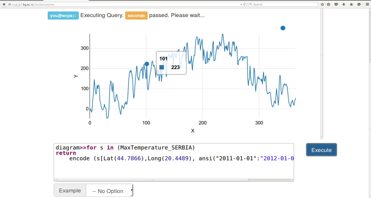
Figure 7.2: Query on the set of spatio-temporal air temperature data for a location with longitude 20.4489 and latitude 44.7866, for every day in 2011.

Another example of a raster database is sciDB.

---